Baseline Representation
As a baseline method, we use the image representations proposed by Vailaya et al. [18]. We selected this approach,
as it reports some of the best results, from all scene classification approaches for datasets with landscape, city and
in door images and since it has already been proven to work on a significant enough dataset. Thus, it can be regarded as
a good representative of the state-of-the-art. Two different representations are used for each binary classification
tasks: color features are used to classify images as indoor or outdoor, and edge features are used to classify outdoor
images as city or landscape. Color features are based on the LUV first- and second-order moments computed over a 10.
Our Representation
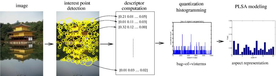
Fig.1 - Representation computation of an image.
There are two main elements in an image classification system. The first one refers to the computation of the
feature vector representing an image, and the second one is the classifier, the algorithm that classifies an input
image into one of the predefined category using the feature vector. In this section, we focus on the image representation
and describe the two models that we use: the first one is the bag-of-visterms, built from automatically extracted and
quantized local descriptors, and the second one is obtained through the higher-level abstraction of the bag-of-visterms
into a set of aspects using the latent space modeling.
Bag-of-visterms representation from local descriptors:
The construction of the bag-of-visterms (BOV) feature vector from an image involves the different steps illustrated in Fig. 1.
In brief, interest points are automatically detected in the image, then local descriptors are computed over those regions.
All the descriptors are quantized into visterms, and all occurrences of each specific visterm of the vocabulary in
the image are counted to build the BOV representation of the image. In the following we describe in more detail each of the steps.
Interest point detection:
The goal of the interest point detector is to automatically extract characteristic points -and more generally regions- from the
image, which are invariant to some geometric and photometric transformations. This invariance property is interesting, as it ensures
that given an image and its transformed version, the same image points will be extracted from both and hence, the same image representation
will be obtained. Several interest point detectors exist in the literature. They vary mostly by the amount of invariance they
theoretically insure, the image property they exploit to achieve invariance, and the type of image structures they are designed to detect [22,23].
In this work, we use the difference of Gaussians (DOG) point detector [22].
This detector essentially identifies blob-like regions where a maximum or minimum of intensity occurs in the image, and it is invariant
to translation, scale, rotation and constant illumination variations.
We chose this detector since it was shown to perform well in comparisons previously published [23]
, and also since we found it to be a good
choice in practice for the task at hand, performing competively compared to other detectors.
The DOG detector is also faster and more compact
than similar performing detectors, and an additional reason to prefer this detector over fully affine-invariant ones [23], is also
motivated by the fact that an increase of the degree of invariance may remove information about the local image content that is valuable for
classification.
Local descriptors:
Local descriptors are computed on the region around each interest point that is automatically identified by the local interest
point detector. We use the SIFT (Scale Invariant Feature Transform) feature as local descriptors [22]. Our choice was motivated by the findings
of several publications [23], where SIFT was found to work best. This descriptor
is based on the grayscale representation of images, and was shown to perform best in terms of specificity of region representation and robustness
to image transformations [23]. SIFT features are local histograms of edge directions computed over different parts of the interest region. These
features capture the structure of the local image regions, which correspond to specific geometric configurations of edges or to more texture-like
content. In [22], it was shown that the use of 8 orientation directions and a grid of 4x4 parts gives a good compromise between descriptor
size and accuracy of representation. The size of the feature vector is thus 128. Orientation invariance is achieved by estimating the dominant
orientation of the local image patch using the orientation histogram of the keypoint region. All direction computations in the elaboration of
the SIFT feature vector are then done with respect to this dominant orientation.
Quantization and Vocabulary model construction:
When applying the two preceding steps to a given image, we obtain a set of real-valued local descriptors. In order to obtain a text-like
representation, we quantize each local descriptor into one of a discrete set of visterms acording to the nearest neighboor rule.
The construction of the vocabulary is performed through clustering. More specifically, we apply the K-means algorithm to a set of
local descriptors extracted from training images, and the means are kept as visterms. We used the Euclidean distance in the clustering
and choose the number of clusters depending on the desired vocabulary size.
Technically, the grouping of similar local descriptors into a specific visterm can be thought of as being similar to the stemming
preprocessing step of text documents, which consists of replacing all words by their stem. The rationale behind stemming is that the meaning
of words is carried by their stem rather than by their morphological variations [24]. The same motivation applies to the quantization
of similar descriptors into a single visterm. Furthermore, in our framework, local descriptors will be considered as distinct whenever
they are mapped to different visterms, regardless of whether they are close or not in the SIFT feature space. This also resembles the
text modeling approach which considers that all information is in the stems, and that any distance defined over their representation
(e.g. strings in the case of text) carries no semantic meaning.
Bag-of-visterms representation:
The first representation of the image that we will use for classification is the bag-of-visterms (BOV), which is constructed from the
local descriptors by counting the occurence in a histogram like fashion. This is equivalent to the bag-of-words representation used
in text documents. This representation of an image contains no information about
spatial relationship between visterms. The standard bag-of-words text representation results in a very similar simplification of the
data: even though word ordering contains a significant amount of information about the original data, it is completely removed from the
final document representation.
Probabilistic Latent Semantic Analysis (PLSA)
The bag-of-words approach has the advantage of producing a simple data representation, but potentially introduces the well known synonymy
and polysemy ambiguities(see analogy with text). Recently, probabilistic latent space models[6] have been proposed
to capture co-occurrence information between elements in a collection of discrete data in order to disambiguate the bag-of-words representation.
The analysis of visterm co-occurrences can thus be considered using similar approaches, and we use the Probabilistic Latent Semantic Analysis
[6] (PLSA) model in this paper for that purpose. Though PLSA suffers from a non-fully generative formulation, its tractable likelihood
maximization makes it an interesting alternative to fully generative models with comparative performance.
Classification Method
To classify an input image represented either by the BOV vectors, the aspect parameters or any of the feature vector of the baseline
approach, we employed Support Vector Machines (SVMs) [25]. SVMs have proven to be successful in solving machine learning problems
in computer vision and text categorization applications, especially those involving large dimensional input spaces. In the current work,
we used Gaussian kernel SVMs, whose bandwidth was chosen based on a 5-fold cross-validation procedure.
Standard SVMs are binary classifiers, for multi-class classification, we adopt a one-against-all approach. Given a n-class problem, we
train n SVMs, where each SVM learns to differentiate images of one class from images of all other classes. In the testing phase, each
test image is assigned to the class of the SVM that delivers the highest output of its decision function.
Protocol
The protocol for each of the classification experiments was as follows. The full dataset of a given experiment was divided into 10
parts, thus defining 10 different splits of the full dataset. One split corresponds to keeping one part of the data for testing, while
using the other nine parts for training (hence the amount of training data is 90% of the full dataset). In this way, we obtain 10 different
classification results. Reported values for all experiments correspond to the average error over all splits, and standard deviations of
the errors are provided in parentheses after the mean value.
Additional experiments were conducted with less amount of training data, to test the robustness of the image representation. In
that case, for each of the splits, images were chosen randomly from the training part of the split to create a reduced training set.
Care was taken to keep the same class proportions in the reduced set as in the original set, and to use the same reduced training set
in those experiments involving two different representation models. The test data of each split was left unchanged.