Representation sparsity

To investigate the analogy with text representation, we compare the behavior between the BOV representation of an image dataset and the bag-of-words representation of a standard text categorization database.

The REUTERS-215781 database contains 9600 training and 3300 testing documents. The standard word stopping and stemming process produces a vocabulary of 17900 words. As previously observed in natural language statistics, the frequency of each word across the text database follows the Zipf s law. This distribution results in an average number of 45 non-zero elements per document, which corresponds to an average sparseness of 0.25%. Out of the 17900 words in the dictionary, 35% occur once in the dataset and 14% occur twice. Only 33% of the words appear in more than five documents.

In our case, we applied the K-means algorithm on the COREL database, which contains 6680 images of city and landscape, and generated the BOV representation for each image document of this database. Since the visterm vocabulary is created by the Kmeans clustering of SIFT descriptors extracted from a set of representative images, the resulting vocabulary shows different properties than in text. The K-means algorithm identifies regions in the feature space containing clusters of points, which prevents the low frequency effect observed in text data. The visterm with the lowest occurrence frequency still occurs in 117 images of the full dataset (0.017 relative frequency). In our experiments, given a vocabulary of 1000 visterms, we observed an average of 175 non-zero elements per image, which corresponds to a data sparseness of 17.5%.

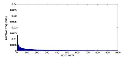
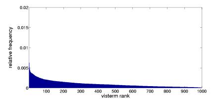
As shown in Fig. 2 (right), the frequency distribution of visterms differs from the Zipf s law behavior usually observed in text.

The construction of the visual vocabulary by clustering intrinsically leads to a flatter distribution for visterms than for words. On one hand, this difference can be considered as an advantage, as the data sparseness observed in the text bag-of-words representation is indeed one of the main problems encountered in text retrieval and categorization. Similar documents might have very different bag-of-words representations because specific words in the vocabulary appear separately in their description. On the other hand, a flatter distribution of the features might imply that, on average, visterms in the visual vocabulary provide less discriminant information. In other words, the semantic content captured by individual visterms is not as specific as the one of words.

Polysemy and synonymy in visterms

To study the semantic nature of the visterms, we first considered the class conditional average of the BOV representation. Fig. 2 (left) shows the average of visterms for the city and landscape scene categories, computed over 250 city images and 400 landscape images. We display the results when using the vocabulary of 100 visterms

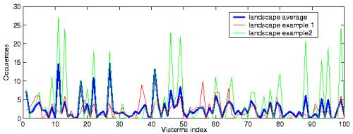
We first notice that there is a large majority of terms that appear in both classes: all the terms are substantially present in the city class; only a few of them do not appear in the landscape class. This contrasts with text documents, in which words are in general more specifically tied to a given category. Furthermore, we can also observe that the major peaks in the two class averages coincide. Thus, when using the BOV representation, the discriminant information with respect to the classification task seems to lie in the difference of average word occurrences. It is worth noticing that this is not due to a bias in the average in visterm numbers, since the difference in the average amount of visterm per class is only in the order of 4% (city 268/ landscape 259). Additionally, these average curves hide the fact that there exists a large variability between samples, as illustrated in Fig. 3 (right), where two random examples are plotted along with the average of the landscape class. Overall, all the above considerations indicate that visterms, taken in isolation, are not so class specific, which in some sense advocates against feature selection based on analysis of the total occurrence of individual features (e.g. [8]), and reflects the fact that the semantic content carried by visterms, if any, is strongly related to polysemy and synonymy issues.

To illustrate that visterms are subject to polysemy -a single visterm may represent different scene content- and synonymy -several visterms may characterize the same image content- consider samples from three different visterms obtained when building the vocabulary, as shown in Fig.3.

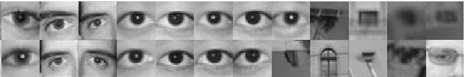
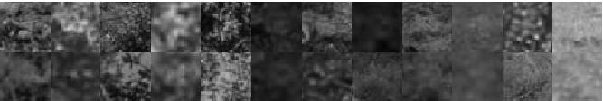
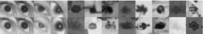
As can be seen, the top visterm represents mostly eyes. However, windows and publicity patches get also indexed by this visterm, which provides an indication of the polysemic nature of that visterm, which means here that although this visterm will mostly occur on faces, it can also occur in city environments. The second row in Fig. 3 present samples from another visterm. Clearly, this visterm also represents eyes, which makes it a synonym of the first displayed visterm. Finally, the samples of a third visterm indicate that this visterm captures a certain fine grain texture that has different origins (rock, trees, road or wall texture...), which illustrates that not all visterms have a clear semantic interpretation. To conclude, it is interesting to notice that one factor that can affect the polysemy and synonymy issue is the vocabulary size: the polysemy of visterms might be more important when using a small vocabulary size than when using a large vocabulary. Conversely, with a large vocabulary, there are more chances to find many synonyms than with a small one.