We present here some selected results to ilustrate the performance of our method. More results can be found in the publications from this project.
Tri-class classification results
| Method | indoor/city/landscape |
| Baseline [18] | 15.9 (1.0) |
| BOV 100 | 12.3 (0.9) |
| BOV 300 | 11.6 (1.0) |
| BOV 600 | 11.5 (0.9) |
| BOV 1000 | 11.1 (0.8) |
Table 1 shows the results of the BOV approach for the three-class classification problem. Classification results were obtained using a multi-class SVM and two binary SVMs in the hierarchical baseline case. We can see that our system outperforms the state-of-the-art approach with statistically significant differences. This is confirmed in all cases by a Paired T-test, for p=0.0001.
Regarding vocabulary size, overall we can see that for vocabularies of 300 visterms or more the classification errors are equivalent. This contrasts with the work in [2], where the flattening of the classification performance was observed only for vocabularies of 1000 visterms or more. A possible explanation may come from the difference in task (object classification) and in the use of the Harris-Affine point detector, known to be less stable than DOG [23]. All of the vocabularies were trained on auxiliar data, this data does not belong to the defined databases for the task, more details on the related publications.
Classification Results using PLSA
In the case of PLSA, we use the probability distribution P(z|d) of latent aspects for each given document. We learn the PLSA models on auxiliar data, this data is not part of the databases that we perform classification on. For more details please read the related publications. Given that PLSA is an unsupervised approach, where no reference to the class label is used during the aspect model learning, we may wonder how much discriminant information remains in the aspect representation. To answer this question, we compare the classification errors obtained with the PLSA and BOV representations.
| Method | Number of aspects | indoor/city/landscape |
| BOV 1000 | 11.1 (0.8) | |
| PLSA | 20 | 12.3 (1.2) |
| PLSA | 60 | 11.9 (1.0) |
Comparing the 60-aspect PLSA model with the BOV approach, we remark that their performance is similar. Learning visual co-occurrences with 60 aspects in PLSA allows for dimensionality reduction by a factor of 17 while keeping the discriminant information contained in the original BOV representation.
Decreasing the amount of training data
Since PLSA captures co-occurrence information from the data it is learned from, it can provide a more stable image representation. We expect this to help in the case of lack of sufficient labeled training data for the classifier. Table 3 compares classification errors for the BOV and the PLSA representations for the tri-class task when using less data to train the SVMs. The amount of training data is given both in proportion to the full dataset size, and as the total number of training images. The test sets remain identical in all cases.
| Method | amount of training data | |||||
| percentage | 90% | 10% | 5% | 2.5% | 1% | |
| number of images | 8511 | 945 | 472 | 236 | 90 | |
| PLSA 60 | 11.9(1.0) | 14.6(1.1) | 15.1(1.4) | 16.7(1.8 | 22.5(4.5) | |
| BOV 1000 | 11.1(0.8) | 15.4(1.1) | 16.6(1.3) | 20.7(1.3) | 31.7(3.4) | |
| Baseline | 15.9(1.0) | 19.7(1.4) | 24.1(1.4) | 29.0(1.6) | 33.9(2.1) | |
Several comments can be made from this table. A general one is that for all methods, the larger the training set, the better the results, showing the need for building large and representative datasets for training (and evaluation) purposes. Qualitatively, with the PLSA and BOV approaches, performance degrades smoothly initially, and degrades sharply when using 1% of training data. With the baseline approach, on the other hand, performance degrades more steadily.
Comparing methods, we can first notice that PLSA with 10% of training data outperforms the baseline approach with full training set (i.e. 90%), this is confirmed a Paired T-test, with p=0.05. More generally, we observe that both PLSA and BOV perform not worse than the baseline for all cases of reduced training set.
Furthermore, we can notice from Table 2 that PLSA deteriorates less as the training set is reduced, producing better results than the BOV approach for all reduced training set experiments (although not always significantly better).
Previous work on probabilistic latent space modeling has reported similar behavior for text data. PLSA's better performance in this case is due to its ability to capture aspects that contain general information about visual co-occurrence. Thus, while the lack of data impairs the simple BOV representation in covering the manifold of documents belonging to a specific scene class (eg. due to the synonymy and polysemy issues) the PLSA-based representation is less affected.
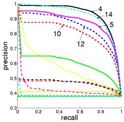
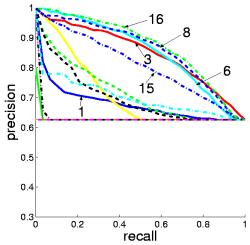
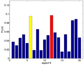
Aspect based image ranking
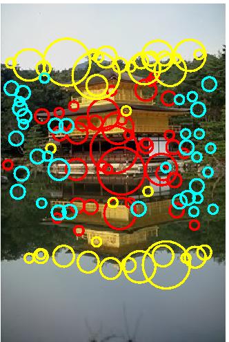
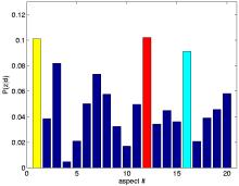
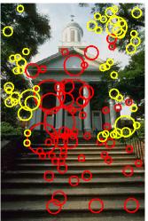
Aspects can be conveniently illustrated by their most probable images in a dataset. Given an aspect z images can be ranked acording to P(z|d). The top-ranked images for a given aspect illustrate its potential semantic meaning. This can be seen in the ranking results.
The top-ranked images representing aspect 1, 6, 8, and 16 all clearly belong to the landscape class. Note that the aspect indices have no intrinsic relevance to a specific class, given the unsupervised nature of the PLSA model learning. Conversely, aspect 4 and 12 are related to the city class.
Considering the aspect-based image ranking as an information retrieval system, the correspondence between aspects and scene classes can be measured objectively. This is done by using the Precision and Recall paired values.